Robert Shiller in his book, Irrational Exuberance, and elsewhere famously argues that due to emotion, stock prices in both bull and bear markets overshoot the prices warranted by future dividends and earnings. If such overshooting occurs, returns on stocks should be negatively Prior Average Dependent (PAD). In particular, lower than normal average returns in the past should be associated with higher than normal returns in the future. If so, negative PAD stock returns should improve the sustainability of disbursements. Persistently lower than expected returns that might otherwise require reductions in disbursements will tend to be offset by higher than originally expected returns in the future.
When historic real returns are regressed on their prior averages the relationship is negative, and becomes more strongly negative as the length of the average increases up to 30 years. Due to inherent bias in such regressions, however, such a negative relationship would be obtained even if the returns are Independently and Identically Distributed (IID) over time. Nevertheless, the regression coefficients obtained could be sufficiently negative to provide evidence that stock returns are negative PAD, and that the results obtained are not just due to bias in the regressions. Such evidence can be provided by simulating a very large number of time series of returns that are known to be IID and are of the same length as the historic series for which the regressions have been made. Regressions can then be run on these simulated series to determine the likelihood of obtaining regression coefficients as negative as those for the historic series when returns are known to be IID. If the coefficients for the historic returns are sufficiently negative to be unlikely to be from IID returns, there is evidence that stock returns are negative PAD, despite the bias. These tests show that there is evidence that stock returns are negative PAD for a 30 year average.
Negative PAD returns affect disbursements both by a hedging benefit, and by the effect of lower or higher than normal average returns before the disbursements begin. To better understand the effect of PAD returns, it is desirable to consider each of these effects separately. The hedging benefit can be isolated by comparing the effect of disbursements from negative PAD stock returns to those from IID stock returns when the returns for the PAD returns before the first disbursement are the same as the expected IID return. To study the effect of the returns prior to the initial disbursement, the returns are set equal to 30 year segments of historical returns. Before doing so, however, the entire historical series is adjusted by the same amount each year so that the average of the historical returns is the same as the expected IID return. The adjusted historic returns prior to 2018 give about the same results as setting the prior returns equal to the expected IID return. Based on the prior 30 year average, the valuation of stocks in 2018 appears to have been about normal. The worst results are obtained for the historic returns prior to the early and mid 1960s that followed the prolonged bullish stock market after WWII. The best results are obtained for returns prior to the mid 1980s that followed the prolonged bearish period in the 1970s and as strong returns in the 1950s were coming out of the 30 year average.
Negative PAD stock returns can affect the optimal allocation to stocks as PAD returns can make stocks more valuable relative to intermediates. When prior returns are equal to the expected IID return, the hedging benefit of PAD returns increases the optimal allocation to stocks by 10 to 20 percentage points depending on the reaction coefficient assumed for the expected return to the prior average. When the prior returns are the high values in the early or mid 1960s, however, it turns out that the adverse effect of these high prior returns offsets the hedging benefit of negative PAD returns. In this case, stocks are no longer more valuable relative to intermediates, and there is no change in the optimal stock allocation from IID stock returns. When the prior stock returns are abnormally low, there is a further increase in the optimal stock allocation beyond that due to the hedging benefit of PAD stock returns.
When initial prior returns are equal to the expected IID return, the hedging benefits of PAD returns provide a meaningful improvement in sustainability. The improvement, however, is not as large as that obtained in the illustration by reducing the initial disbursement from 4.0% to 3.5% for IID returns. More improvement than reducing the initial disbursement from 4.0% to 3.5% can be obtained, however, when the initial prior returns are as low as have been observed historically. When the initial prior returns are as high as have been observed historically the deterioration in sustainability is serious, but not as bad as increasing the initial disbursement from 4.0% to 4.5% in the illustration for IID returns. Thus, PAD stock returns provide a meaningful benefit for normal initial prior returns such as those that existed in 2018. Much larger benefits occur when prior returns are as low as sometimes in the past. Serious deterioration in sustainability occurs when prior returns are as high as have sometimes been observed.
Evidence
The 2018 SBBI Yearbook has a well-known series of annual real returns for large capitalization stocks from 1926 to 2017. These returns are identical to those for the S&P 500 starting in the late 1950s when the S&P 500 was introduced. To use this series to provide a prior average as long as 40 years, the first year that can be used for a regression of these returns on their prior averages is 1966. The results of such regressions for the returns from 1966 to 2017 on their prior moving averages are shown in Table 3. The regression coefficients are negative and become more strongly negative as the length of the moving average increases to 30 years. As just noted, however, such regressions have a bias to give negative coefficients even if the returns in the series are not negative PAD, but IID. There is a negative bias because having a prior moving average above its own average over the sample period makes it more likely that subsequent returns in the sample period are below average and this tendency is stronger the longer is the moving average. On the other hand, having a prior moving average below its own average makes it more likely that subsequent returns are above average so that there is negative covariance between returns in a sample period and a prior moving average even if those returns are IID.
The negative bias can be confirmed and its size investigated by running regressions on simulated time series of returns that are IID. To do so, suppose that 50,000 time series of returns are simulated that are of the same length as the series of historic returns that were used to obtain the results in Table 3. Suppose also that these returns are IID with a normal distribution with a mean of .07 and a standard deviation of .18. Results from these regressions are shown in the two columns on the right of Table 3. The chances that the regression coefficients are negative increase from .74 for a 10 year average to .87 for a 40 year average. The column on the far right shows that regression coefficients as negative as those obtained for the historic returns with shorter averages could easily be due to chance if the underlying returns are IID. Coefficients as negative as those obtained for the longer averages, however, are less likely to be due to chance. In particular, the coefficient for the 30 year average has only a .035 chance of occurring if the returns are IID, which is less than the .05 chance often used for establishing significance. Perhaps, however, the coefficient for the 30 year average is unlikely because the underlying stock returns have a different mean or standard deviation than assumed for the IID returns. When the mean or standard deviation is varied by .02, however, virtually the same results are obtained as in the two columns on the right of Table 3. It is of interest to note, but not necessarily of much consequence, that the lowest and highest 30 year averages over 1966 to 2017 occurred just prior to the unusually strong bull market of 1995/99, and the unusually severe bear market of 1973/74.(1)
Modelling
To illustrate negative PAD returns the return each year is assumed to be a linear function of the prior moving average of the returns plus an independently distributed random variable with a zero mean, just like the regressions. As an average of 30 years gives the best results, a 30 year average will be used. To allow for the bias and be reasonably conservative, a value of —1 will be used for the coefficient of the 30 year average, but a coefficient of -2 will also be tested. When the coefficient is —1, the constant term of the linear relation is set equal to .14 so that the expected return is equal to .07 when the prior average return is .07. Likewise, when the coefficient is equal to —2, the constant term is set equal to .21 so that the expected return is equal to .07 in this case when the average is equal to .07. The independent random component of the return each year is assumed to be normally distributed. The moving averages are then also normally distributed because they are linear functions of normally distributed variables, and the returns each year are normally distributed like the IID returns. Some modifications required to include PAD stock returns in the formal Model are discussed in a note.(2)
To evaluate the effect of the negative PAD returns on sustainability, it is desirable to first consider returns that are otherwise as similar to the IID returns as possible. At the beginning of the first year, for the IID returns, the expected value of all the future returns is .07, and their standard deviation is .18. For the negative PAD returns, all of the future expected returns at the beginning of the first year will also equal .07 if and only if each of the 30 prior returns equals .07. In this case, an expected return of .07 is both added and deducted from the moving average each year keeping the expected return and expected average both equal to .07. This will not be true unless all of the prior returns are equal to .07.
Suppose the standard deviation of the independent random component of the PAD returns each year is set equal to .18. In this case, viewed from the beginning of the first year, only the standard deviation of the return for the first year will then be equal to .18. The volatility of the following returns will be higher than .18 due to random variation in the moving average. For instance, for the second year, the variability of the moving average adds a fraction equal to (1/30) squaredof the variance of the return for the first year to the variance of the return for the second year, making the standard deviation equal to .18010. For the third year, the effect of variation in the returns for both the first and second years on the moving average further increases the standard deviation to .18019.
For years further in the future the calculations become more complex, but sufficiently accurate results can be obtained by simulation. By year 36 the standard deviation has increased to about .1815. Viewed from the beginning of the first year the increase in volatility versus the IID returns is very small. To further reduce the difference, and better identify the hedging benefit of the negative PAD returns, the standard deviation of the independent component of the returns can be reduced somewhat below .18 so that the average volatility of these returns over time is very close to .18. Similar considerations apply when intermediates are included in the portfolio, and are discussed in a note.(3)
Results
Viewed from the beginning of the first year, for prior returns equal to the assumed expected IID return of .07, all of the future expected returns are equal to .07. Viewed from the beginning of a future year, however, the expected return for that future year depends on whatever the prior average return happens to be at that time. The distribution of the expected returns viewed from the beginning of a future year can be determined by obtaining the distribution of the moving average for that year with simulations. The distributions of the expected returns at the beginning of future years, as viewed from the beginning of the first year, are shown in Chart 24 for initial prior returns equal to .07, and a coefficient of —1. For the 5% of cases where the returns are very low in the early years, and reductions in the disbursements are likely to be required, note that the expected return has increased from .07 to .10 or more by year 15. If the coefficient is instead set equal to —2, the expected return in 15 years increases from .07 to .12 or more.
With negative PAD stock returns, very low returns in the early years that may require future reductions in the disbursements result in higher expected returns that will reduce any such reductions. The more negative is the coefficient of the average, the stronger is the hedge provided by PAD stock returns. Due to this hedge, stocks become more valuable relative to intermediates increasing the optimal allocation to stocks. Allocation shows for a 3.5% initial disbursement with IID returns that a 30% allocation to stocks provides cumulative probability distributions for future disbursements that are to the right of those for either lower or higher stock allocations. Similar results occur at years 12, 24, and 36 so that looking at year 24 is sufficient. When stocks are PAD with a coefficient of —1 for the average, Chart 25 shows that similar results are obtained when the stock allocation is increased from 30% to 40%. Thus, when the coefficient is —1 the optimal stock allocation increases to 40%. When the coefficient is —2, Chart 26 shows that the optimal stock allocation increases further to 50%. These increases in the allocation to stocks assume the initial prior returns are reasonably normal. The effect of highly unusual prior returns on allocation are discussed in the next section. Allocation shows for IID returns that the optimal stock allocation increases by 10 percentage points when the initial disbursement increases from 3.5% to 4.5%. Such an increase is also applicable for PAD stock returns. The RDR in all cases is the expected return for the allocation based on the .03 expected return for the intermediates and an assumed expected return of .07 for the stocks.
The effect of PAD returns on sustainability will be investigated by looking at a typical situation. Increase shows that a 4.0% initial disbursement has a .22 chance of a decline by year 24 using the illustration for IID returns. Suppose the IID returns are replaced by PAD returns, and that the initial prior returns are equal to the expected IID return. The dashed curves in Chart 27 show that the chances of a decline drop from .22 to from .12 to .16, depending on whether the reaction coefficient for expected return to the 30 year average is assumed to be —1 or —2. The hedging benefit provides a meaningful improvement in sustainability. As a comparison, however, this improvement is well short of the reduction from .22 to .08 provided for IID returns when the initial disbursement is reduced from 4.0% to 3.5%. The next section shows, however, that reductions below .08 are obtained with PAD returns when the initial prior disbursements are not normal, but at the low end of the range that has been observed historically.
Initial Prior Returns
So far, the initial prior returns have been set equal to the expected IID return. Now suppose that the prior returns are the most recent 30 annual real returns in the 1926 to 2017 historical series, or the 30 consecutive returns in that series that would have an unusually strong impact either positive or negative on sustainability. To have a strong impact on sustainability the prior average must be unusually low or high and more recent returns should also be unusually low or high as recent returns will remain in the average for a long time. Unusually high averages with more recent high returns occurred prior to the early and mid 1960s following the long bullish period in the stock market after WWII. In particular, the returns prior to 1966 will be considered as that is the first year for the regressions in Table 3. An unusually low average with more recent low returns occurred in the mid 1980s following the long bearish period in the stock market in the 1970s. The mid 1980s also reflects some of the unusually strong returns in the 1950s coming out of the 30 year average. In particular, the returns prior to 1985 will be considered. To isolate the effect of the pattern of the returns in the historical series from the difference between the average historical returns and the expected IID return, an adjustment is required. All of the returns in the historical series must be adjusted by the same amount so that the average return of the historical series is the same as the expected IID return. To do so, each of the historical returns must be reduced by .020, as the average return over 1926 to 2017 was .090.
For normal initial prior returns the hedging benefit of PAD returns makes stocks more valuable relative to intermediates, and increases the allocation to stocks by 10 or 20 percentage points for the illustration. This advantage for stocks with PAD returns can be nullified, however, if the initial prior returns are too high. Suppose, for instance, that the initial prior stock returns are those in 1966, after the adjustment just described. When the prior returns for 1966 replace the prior returns of .07 in Chart 25, Chart 28 shows that the optimal stock allocation reverts from 40% back to 30% for a coefficient of —1. When the coefficient is —2, the reversion is from 50% to 30%. The stronger reaction coefficient strengthens the hedging benefit, but also strengthens the adverse effect of the very high prior returns. The net effect is no change. When the prior returns are replaced by the very low prior returns in 1985, the prior returns increase the allocation from 40% to 50% for a coefficient of —1, and to 60% for a coefficient of —2. All of these allocations are for a 3.5% initial disbursement, and as before, an increase in the initial disbursement to 4.0% or 4.5% warrants adding 5 or 10 percentage points to the allocation. Change in the 30 year average return as the disbursement period unfolds might make some later change in allocation desirable, but doing so will not have much effect on sustainability, and will not be considered.
When the initial prior returns are equal to .07, PAD stock returns reduce the chance of a decline in a 4.0% initial disbursement by year 24 from .22 to from .16 to .12 depending on whether the reaction coefficient for the prior average is —1 or —2. Table 4 shows comparable results when the 30 initial prior annual real returns are the adjusted historical returns prior to 2018, 1985, and 1966. In 2018 the adjusted 30 year average was .073, and thus slightly above .07. The 2018 priors, however, do not give slightly worse sustainability as might be expected, but provide a small improvement. Note that the pattern as well as the average of the prior returns matters with respect to future performance. The 30 years prior to 2018, for instance, includes the unusually strong bull market of 1995/99. Those strong returns, however, soon come out of the 30 year average.
In any case, the adjusted priors in 2018 were close to normal, and give results very similar to priors equal to the expected IID return. Based on the 30 year average, the valuation of stocks in 2018 appears to have been close to normal. Table 4 shows, however, that the priors for 1985 and 1966 give very different results. The priors for 1985 reduce the chances for a decline to from .01 to .06. These chances are less than the .08 chance of a decline obtained by reducing the initial disbursement for IID returns from 4.0% to 3.5%. The priors for 1966 increase the chances of a decline to from .30 to .38. These chances are less than, but nevertheless close to, the .40 chance of a decline obtained by increasing the initial disbursement from 4.0% to 4.5% for IID returns. The declines for a 4.0% initial disbursement at year 24 are compared in Chart 29 for the priors at years 2018, 1985, and 1966. In general, PAD stock returns provide a meaningful improvement for normal prior returns such as those that existed in 2018. Much larger benefits occur when prior returns are as low as have been observed in the past. Serious deterioration in sustainability occurs when initial prior returns are as high as have been observed in the past.
Notes
Over 1966 to 2017, the strongest bull market was over 1995 to 1999 when the annual increase for those five years averaged 26% in real terms. The most severe bear market was over 1973 and 1974 when the annual decline averaged 28% in real terms for these two years. It is of interest to note that the trough and peak of the 30 year average over 1966 to 2017 occurred in the year just prior to each of these events. Of course, there was no way of knowing that was the peak or trough until long afterwards. Moreover, for many years beforehand the 30 year average was almost as low or as high as at the trough or peak. Thus, the 30 year average would not have been of much help in forecasting the timing of these events. Highly abnormal measures of stock market valuation are helpful in indicating that a highly abnormal move of the market is possible, not when it will occur
To incorporate PAD stock returns into the Model, two new columns must be added to the spreadsheet, and a revision made in the relation for the stock return, r(t). The first of the new columns has the 65 returns that are used in each iteration for a simulation of the disbursements. The first 30 of these returns starts with the most distant of the 30 given prior returns, and ends with the given return for the year prior to the beginning of the disbursements. The last 35 returns start with the drawing for the return for the first year in the iteration, and end with the drawing for the return for the 35th year in that iteration. The second column has the 36 successive moving averages of the 30 prior returns used to calculate the expected return for each successive year in an iteration. The first of these is the average of the 30 given prior returns, and the last is the 30 returns drawn in the simulation for the 6th through the 35th years of an iteration. In the relation for the return on stocks in year t given by r(t), the mean is increased by .07, when the coefficient is —1, and the prior average for year t given in the second column deducted. When the coefficient is —2, .14 is added to the mean and twice the prior average for year t given in the second column is deducted. As discussed in the following note, when the coefficients are —1 and —2 the standard deviation is set respectively to .1768 and .1758.
For the IID stock returns suppose that intermediate term fixed income issues are included in the portfolio. The annual real returns on the intermediates are independently distributed over time with an identical normal distribution each year that has a mean of .03 and a standard deviation of .07. The annual real return for the stocks each year is equal to .4 of the real return of the intermediates for that year plus an independently distributed normal variable with a mean and standard deviation set to keep the expected return on the stocks each year equal to .07 and the standard deviation equal to .18. Setting the mean and standard deviation of the independent random variable equal respectively to .058 and ,1778 does this when the stock returns are IID. When the stock returns are PAD with a coefficient of —1 or —2 for the prior 30 year average, .07 and .14 must be added respectively to .058 to keep the expected return of the stocks equal to .07 when the average is equal to .07 with those values for the coefficient of the average. If the standard deviation of the independent random component is set equal to .1778, the standard deviation of the stock returns for the first year is .18. As discussed in the text without the intermediates, however, the standard deviation rises somewhat in the future due to the random variation in the moving average component of PAD stock returns. To make the average standard deviation over time of the returns on the stocks about equal to .18 with the intermediates, the standard deviation of the independent random component must be reduced from .1778 to .1768 when the coefficient is —1, and to .1758 when the coefficient is —2. Simulations confirm that the average standard deviation of the stock returns over time is then about .18.
References
Duff & Phelps, 2018 SBBI Yearbook, New York, 2018.
Robert J. Shiller, Irrational Exuberance, Princeton University Press, Princeton, NJ, 2000.
PAD
PAD Stock Returns
Robert Shiller in his book, Irrational Exuberance, and elsewhere famously argues that due to emotion, stock prices in both bull and bear markets overshoot the prices warranted by future dividends and earnings. If such overshooting occurs, returns on stocks should be negatively Prior Average Dependent (PAD). In particular, lower than normal average returns in the past should be associated with higher than normal returns in the future. If so, negative PAD stock returns should improve the sustainability of disbursements. Persistently lower than expected returns that might otherwise require reductions in disbursements will tend to be offset by higher than originally expected returns in the future.
When historic real returns are regressed on their prior averages the relationship is negative, and becomes more strongly negative as the length of the average increases up to 30 years. Due to inherent bias in such regressions, however, such a negative relationship would be obtained even if the returns are Independently and Identically Distributed (IID) over time. Nevertheless, the regression coefficients obtained could be sufficiently negative to provide evidence that stock returns are negative PAD, and that the results obtained are not just due to bias in the regressions. Such evidence can be provided by simulating a very large number of time series of returns that are known to be IID and are of the same length as the historic series for which the regressions have been made. Regressions can then be run on these simulated series to determine the likelihood of obtaining regression coefficients as negative as those for the historic series when returns are known to be IID. If the coefficients for the historic returns are sufficiently negative to be unlikely to be from IID returns, there is evidence that stock returns are negative PAD, despite the bias. These tests show that there is evidence that stock returns are negative PAD for a 30 year average.
Negative PAD returns affect disbursements both by a hedging benefit, and by the effect of lower or higher than normal average returns before the disbursements begin. To better understand the effect of PAD returns, it is desirable to consider each of these effects separately. The hedging benefit can be isolated by comparing the effect of disbursements from negative PAD stock returns to those from IID stock returns when the returns for the PAD returns before the first disbursement are the same as the expected IID return. To study the effect of the returns prior to the initial disbursement, the returns are set equal to 30 year segments of historical returns. Before doing so, however, the entire historical series is adjusted by the same amount each year so that the average of the historical returns is the same as the expected IID return. The adjusted historic returns prior to 2018 give about the same results as setting the prior returns equal to the expected IID return. Based on the prior 30 year average, the valuation of stocks in 2018 appears to have been about normal. The worst results are obtained for the historic returns prior to the early and mid 1960s that followed the prolonged bullish stock market after WWII. The best results are obtained for returns prior to the mid 1980s that followed the prolonged bearish period in the 1970s and as strong returns in the 1950s were coming out of the 30 year average.
Negative PAD stock returns can affect the optimal allocation to stocks as PAD returns can make stocks more valuable relative to intermediates. When prior returns are equal to the expected IID return, the hedging benefit of PAD returns increases the optimal allocation to stocks by 10 to 20 percentage points depending on the reaction coefficient assumed for the expected return to the prior average. When the prior returns are the high values in the early or mid 1960s, however, it turns out that the adverse effect of these high prior returns offsets the hedging benefit of negative PAD returns. In this case, stocks are no longer more valuable relative to intermediates, and there is no change in the optimal stock allocation from IID stock returns. When the prior stock returns are abnormally low, there is a further increase in the optimal stock allocation beyond that due to the hedging benefit of PAD stock returns.
When initial prior returns are equal to the expected IID return, the hedging benefits of PAD returns provide a meaningful improvement in sustainability. The improvement, however, is not as large as that obtained in the illustration by reducing the initial disbursement from 4.0% to 3.5% for IID returns. More improvement than reducing the initial disbursement from 4.0% to 3.5% can be obtained, however, when the initial prior returns are as low as have been observed historically. When the initial prior returns are as high as have been observed historically the deterioration in sustainability is serious, but not as bad as increasing the initial disbursement from 4.0% to 4.5% in the illustration for IID returns. Thus, PAD stock returns provide a meaningful benefit for normal initial prior returns such as those that existed in 2018. Much larger benefits occur when prior returns are as low as sometimes in the past. Serious deterioration in sustainability occurs when prior returns are as high as have sometimes been observed.
Evidence
The 2018 SBBI Yearbook has a well-known series of annual real returns for large capitalization stocks from 1926 to 2017. These returns are identical to those for the S&P 500 starting in the late 1950s when the S&P 500 was introduced. To use this series to provide a prior average as long as 40 years, the first year that can be used for a regression of these returns on their prior averages is 1966. The results of such regressions for the returns from 1966 to 2017 on their prior moving averages are shown in Table 3. The regression coefficients are negative and become more strongly negative as the length of the moving average increases to 30 years. As just noted, however, such regressions have a bias to give negative coefficients even if the returns in the series are not negative PAD, but IID. There is a negative bias because having a prior moving average above its own average over the sample period makes it more likely that subsequent returns in the sample period are below average and this tendency is stronger the longer is the moving average. On the other hand, having a prior moving average below its own average makes it more likely that subsequent returns are above average so that there is negative covariance between returns in a sample period and a prior moving average even if those returns are IID.
The negative bias can be confirmed and its size investigated by running regressions on simulated time series of returns that are IID. To do so, suppose that 50,000 time series of returns are simulated that are of the same length as the series of historic returns that were used to obtain the results in Table 3. Suppose also that these returns are IID with a normal distribution with a mean of .07 and a standard deviation of .18. Results from these regressions are shown in the two columns on the right of Table 3. The chances that the regression coefficients are negative increase from .74 for a 10 year average to .87 for a 40 year average. The column on the far right shows that regression coefficients as negative as those obtained for the historic returns with shorter averages could easily be due to chance if the underlying returns are IID. Coefficients as negative as those obtained for the longer averages, however, are less likely to be due to chance. In particular, the coefficient for the 30 year average has only a .035 chance of occurring if the returns are IID, which is less than the .05 chance often used for establishing significance. Perhaps, however, the coefficient for the 30 year average is unlikely because the underlying stock returns have a different mean or standard deviation than assumed for the IID returns. When the mean or standard deviation is varied by .02, however, virtually the same results are obtained as in the two columns on the right of Table 3. It is of interest to note, but not necessarily of much consequence, that the lowest and highest 30 year averages over 1966 to 2017 occurred just prior to the unusually strong bull market of 1995/99, and the unusually severe bear market of 1973/74.(1)
Modelling
To illustrate negative PAD returns the return each year is assumed to be a linear function of the prior moving average of the returns plus an independently distributed random variable with a zero mean, just like the regressions. As an average of 30 years gives the best results, a 30 year average will be used. To allow for the bias and be reasonably conservative, a value of —1 will be used for the coefficient of the 30 year average, but a coefficient of -2 will also be tested. When the coefficient is —1, the constant term of the linear relation is set equal to .14 so that the expected return is equal to .07 when the prior average return is .07. Likewise, when the coefficient is equal to —2, the constant term is set equal to .21 so that the expected return is equal to .07 in this case when the average is equal to .07. The independent random component of the return each year is assumed to be normally distributed. The moving averages are then also normally distributed because they are linear functions of normally distributed variables, and the returns each year are normally distributed like the IID returns. Some modifications required to include PAD stock returns in the formal Model are discussed in a note.(2)
To evaluate the effect of the negative PAD returns on sustainability, it is desirable to first consider returns that are otherwise as similar to the IID returns as possible. At the beginning of the first year, for the IID returns, the expected value of all the future returns is .07, and their standard deviation is .18. For the negative PAD returns, all of the future expected returns at the beginning of the first year will also equal .07 if and only if each of the 30 prior returns equals .07. In this case, an expected return of .07 is both added and deducted from the moving average each year keeping the expected return and expected average both equal to .07. This will not be true unless all of the prior returns are equal to .07.
Suppose the standard deviation of the independent random component of the PAD returns each year is set equal to .18. In this case, viewed from the beginning of the first year, only the standard deviation of the return for the first year will then be equal to .18. The volatility of the following returns will be higher than .18 due to random variation in the moving average. For instance, for the second year, the variability of the moving average adds a fraction equal to (1/30) squared of the variance of the return for the first year to the variance of the return for the second year, making the standard deviation equal to .18010. For the third year, the effect of variation in the returns for both the first and second years on the moving average further increases the standard deviation to .18019.
For years further in the future the calculations become more complex, but sufficiently accurate results can be obtained by simulation. By year 36 the standard deviation has increased to about .1815. Viewed from the beginning of the first year the increase in volatility versus the IID returns is very small. To further reduce the difference, and better identify the hedging benefit of the negative PAD returns, the standard deviation of the independent component of the returns can be reduced somewhat below .18 so that the average volatility of these returns over time is very close to .18. Similar considerations apply when intermediates are included in the portfolio, and are discussed in a note.(3)
Results
Viewed from the beginning of the first year, for prior returns equal to the assumed expected IID return of .07, all of the future expected returns are equal to .07. Viewed from the beginning of a future year, however, the expected return for that future year depends on whatever the prior average return happens to be at that time. The distribution of the expected returns viewed from the beginning of a future year can be determined by obtaining the distribution of the moving average for that year with simulations. The distributions of the expected returns at the beginning of future years, as viewed from the beginning of the first year, are shown in Chart 24 for initial prior returns equal to .07, and a coefficient of —1. For the 5% of cases where the returns are very low in the early years, and reductions in the disbursements are likely to be required, note that the expected return has increased from .07 to .10 or more by year 15. If the coefficient is instead set equal to —2, the expected return in 15 years increases from .07 to .12 or more.
With negative PAD stock returns, very low returns in the early years that may require future reductions in the disbursements result in higher expected returns that will reduce any such reductions. The more negative is the coefficient of the average, the stronger is the hedge provided by PAD stock returns. Due to this hedge, stocks become more valuable relative to intermediates increasing the optimal allocation to stocks. Allocation shows for a 3.5% initial disbursement with IID returns that a 30% allocation to stocks provides cumulative probability distributions for future disbursements that are to the right of those for either lower or higher stock allocations. Similar results occur at years 12, 24, and 36 so that looking at year 24 is sufficient. When stocks are PAD with a coefficient of —1 for the average, Chart 25 shows that similar results are obtained when the stock allocation is increased from 30% to 40%. Thus, when the coefficient is —1 the optimal stock allocation increases to 40%. When the coefficient is —2, Chart 26 shows that the optimal stock allocation increases further to 50%. These increases in the allocation to stocks assume the initial prior returns are reasonably normal. The effect of highly unusual prior returns on allocation are discussed in the next section. Allocation shows for IID returns that the optimal stock allocation increases by 10 percentage points when the initial disbursement increases from 3.5% to 4.5%. Such an increase is also applicable for PAD stock returns. The RDR in all cases is the expected return for the allocation based on the .03 expected return for the intermediates and an assumed expected return of .07 for the stocks.
The effect of PAD returns on sustainability will be investigated by looking at a typical situation. Increase shows that a 4.0% initial disbursement has a .22 chance of a decline by year 24 using the illustration for IID returns. Suppose the IID returns are replaced by PAD returns, and that the initial prior returns are equal to the expected IID return. The dashed curves in Chart 27 show that the chances of a decline drop from .22 to from .12 to .16, depending on whether the reaction coefficient for expected return to the 30 year average is assumed to be —1 or —2. The hedging benefit provides a meaningful improvement in sustainability. As a comparison, however, this improvement is well short of the reduction from .22 to .08 provided for IID returns when the initial disbursement is reduced from 4.0% to 3.5%. The next section shows, however, that reductions below .08 are obtained with PAD returns when the initial prior disbursements are not normal, but at the low end of the range that has been observed historically.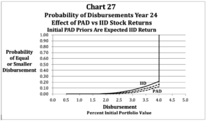
Initial Prior Returns
So far, the initial prior returns have been set equal to the expected IID return. Now suppose that the prior returns are the most recent 30 annual real returns in the 1926 to 2017 historical series, or the 30 consecutive returns in that series that would have an unusually strong impact either positive or negative on sustainability. To have a strong impact on sustainability the prior average must be unusually low or high and more recent returns should also be unusually low or high as recent returns will remain in the average for a long time. Unusually high averages with more recent high returns occurred prior to the early and mid 1960s following the long bullish period in the stock market after WWII. In particular, the returns prior to 1966 will be considered as that is the first year for the regressions in Table 3. An unusually low average with more recent low returns occurred in the mid 1980s following the long bearish period in the stock market in the 1970s. The mid 1980s also reflects some of the unusually strong returns in the 1950s coming out of the 30 year average. In particular, the returns prior to 1985 will be considered. To isolate the effect of the pattern of the returns in the historical series from the difference between the average historical returns and the expected IID return, an adjustment is required. All of the returns in the historical series must be adjusted by the same amount so that the average return of the historical series is the same as the expected IID return. To do so, each of the historical returns must be reduced by .020, as the average return over 1926 to 2017 was .090.
For normal initial prior returns the hedging benefit of PAD returns makes stocks more valuable relative to intermediates, and increases the allocation to stocks by 10 or 20 percentage points for the illustration. This advantage for stocks with PAD returns can be nullified, however, if the initial prior returns are too high. Suppose, for instance, that the initial prior stock returns are those in 1966, after the adjustment just described. When the prior returns for 1966 replace the prior returns of .07 in Chart 25, Chart 28 shows that the optimal stock allocation reverts from 40% back to 30% for a coefficient of —1. When the coefficient is —2, the reversion is from 50% to 30%. The stronger reaction coefficient strengthens the hedging benefit, but also strengthens the adverse effect of the very high prior returns. The net effect is no change. When the prior returns are replaced by the very low prior returns in 1985, the prior returns increase the allocation from 40% to 50% for a coefficient of —1, and to 60% for a coefficient of —2. All of these allocations are for a 3.5% initial disbursement, and as before, an increase in the initial disbursement to 4.0% or 4.5% warrants adding 5 or 10 percentage points to the allocation. Change in the 30 year average return as the disbursement period unfolds might make some later change in allocation desirable, but doing so will not have much effect on sustainability, and will not be considered.
When the initial prior returns are equal to .07, PAD stock returns reduce the chance of a decline in a 4.0% initial disbursement by year 24 from .22 to from .16 to .12 depending on whether the reaction coefficient for the prior average is —1 or —2. Table 4 shows comparable results when the 30 initial prior annual real returns are the adjusted historical returns prior to 2018, 1985, and 1966. In 2018 the adjusted 30 year average was .073, and thus slightly above .07. The 2018 priors, however, do not give slightly worse sustainability as might be expected, but provide a small improvement. Note that the pattern as well as the average of the prior returns matters with respect to future performance. The 30 years prior to 2018, for instance, includes the unusually strong bull market of 1995/99. Those strong returns, however, soon come out of the 30 year average.
In any case, the adjusted priors in 2018 were close to normal, and give results very similar to priors equal to the expected IID return. Based on the 30 year average, the valuation of stocks in 2018 appears to have been close to normal. Table 4 shows, however, that the priors for 1985 and 1966 give very different results. The priors for 1985 reduce the chances for a decline to from .01 to .06. These chances are less than the .08 chance of a decline obtained by reducing the initial disbursement for IID returns from 4.0% to 3.5%. The priors for 1966 increase the chances of a decline to from .30 to .38. These chances are less than, but nevertheless close to, the .40 chance of a decline obtained by increasing the initial disbursement from 4.0% to 4.5% for IID returns. The declines for a 4.0% initial disbursement at year 24 are compared in Chart 29 for the priors at years 2018, 1985, and 1966. In general, PAD stock returns provide a meaningful improvement for normal prior returns such as those that existed in 2018. Much larger benefits occur when prior returns are as low as have been observed in the past. Serious deterioration in sustainability occurs when initial prior returns are as high as have been observed in the past.
Notes
References
Duff & Phelps, 2018 SBBI Yearbook, New York, 2018.
Robert J. Shiller, Irrational Exuberance, Princeton University Press, Princeton, NJ, 2000.
Posted March 2019